Analytical Evolutionary Model for Protein Fold Occurrence in Genomes, Accounting for the Effects of Gene Duplication, Deletion, Acquisition and Selective Pressure

Motivation

Global surveys of protein folds in genomes measure the usage of essential molecular parts in different organisms. In a recent survey, we showed that the occurrence of protein folds in 20 completely sequence genomes follow a power-law distribution; i.e., the number of folds (F) with a given genomic occurrence (V) decays as F (V )= aV ^-b, with a few occurring many times and most occurring infrequently. Clearly, such a distribution results from the way in which genomes have evolved into their current states.

Results

Here we develop and discuss a minimal, analytically tractable model to explain these observations. In particular, we demonstrate that (i) stochastic gene duplication and (ii) overall acquisition of new folds are sufficient to accurately replicate the power-law distributions. Furthermore by optimizing the model using genomic data, we gain a quantitative insight into otherwise unattainable data. In particular, as the rate at which genomes acquire new folds is directly related to the power-law exponent-b, we can easily estimate this rate by measuring the gradient of the distribution on a log-log graph. In addition, extensions to the model suggest that gene deletion and selective pressure are important to the fate of individual genes, but do not significantly affect the final power-law distribution. That is, although gene deletion and selective pressure will affect the choice of the most common fold type in an organism, it will not change the overall power-law distribution found across different genomes. Finally, we gain an indication of the initial sizes of genomes, from the starting states of the simulations. We find that the power-law dependence of the fold distribution is independent of the composition of the starting genome.

Availability

Additional data pertaining to this work is found at http://www.partslist.org/powerlaw.

Introduction

The power-law behavior is frequently found in many different population distributions. Also referred to as Zipf 's law, a well-documented example is the usage of words in text documents.¹ By grouping words that have similar occurrences, it was noted that a small selection such as “the” and “of ” are used many times, while most occur infrequently. When the size of each group is plot against its usage, the distribution is described by a power-law function: the number of words (F) with a given occurrence (V) decays with the equation F = a/V ^-b. The distribution is linear when plot on log-log axes, where-b describes the slope. Such distributions are also found for the relative sizes of cities, income levels and the number of papers published by scientists in a field of research.¹

Significantly, the power-law behavior is also prevalent in many aspects of genomic biology. ² It is found in the usage of short nucleotide sequences,^3-7 the populations of gene families,^8,9 the occurrence of protein superfamilies and folds in genomes^10,11 and several biological networks.^12-14 The distribution extends even further to the number of distinct protein functions associated with a particular fold, the number of protein-protein interactions that are made by each fold type, and the variations in expression levels between genes present in the yeast genome. These observations have been made in at least 20 prokaryotic and eukaryotic genomes, and so are likely to be universal to most other genomes that are yet to be analyzed. Given the prevalence of this behavior, we suggest that all of these biological distributions arise because of a common mechanism for genomic evolution, primarily by duplicating existing genes to increase the presence of particular types of proteins.¹¹

The current study focuses on the distribution of protein folds in different organisms (fig. 1A). Most proteins encoded in a genome have a defined three-dimensional structure that can be classified into distinct protein folds. Although these folds are defined by the topology of the peptide chain, it is possible to determine whether two proteins adopt the same fold by sequence comparison. So even if structures are unavailable for all the genes, we can classify them into equivalent folds by sequence similarity. Using these classifications, one way of representing the contents of a genome is to count the number of times different folds occur and then group together those with similar occurrences (fig. 1B). Like word usage, the number of folds (F) with a certain genomic occurrence (V) decays according to the power-law function; we display the distribution for the E. coli genome in Figure 1A, and plots for 19 further organisms is available from our supplementary website.

Figure 1

The occurrence of protein folds in genomes. A) The structural contents of a genome can be represented by counting the number of times different protein folds occur and grouping together those with similar occurrences. B) The relationship is described (more...)

There have been several efforts to understand this nonuniform distribution of protein families. A number of models suggested that the observation of non-uniform population distributions of protein families depends on the ”designability” of the protein structure; that is, the relative size of a family depends on the fraction of all sequences that could successfully fold into any particular protein fold.^15,16 Others have modelled the occurrence of non-uniform distributions by simulating the evolution of genomes. In the model of Huynen and van Nimwegen,⁹ families expand or shrink in size through successive multiplications by a random factor, which represents duplication or deletion events depending on its value. More recently, Yanai et al¹⁷ introduced a model in which a genome evolves from a set of precursor genes to a mature size by iterative gene duplications and gradual accumulation of modifications through point mutations. When an individual family member acquires enough random mutations, it breaks away to form a new family.

We recently presented an equally minimal, but more biologically realistic model.¹¹ Here genomes evolve through stochastic gene duplications and steady acquisition of new protein folds, either by ab initio creation or horizontal gene transfer.^18-22 Simulations replicated the genomic distributions very accurately, and provided insight into the rate at which different organisms acquired new folds and the origins of a common ancestral genome. Although our work focused on the distribution of protein fold populations, the model applied equally well for other gene classifications such as sequence families, and SCOP superfamilies.²³ The behavior also applies for alternative protein classification systems such as Interpro families and protein superfamilies.

The purpose of the current work is two-fold. First, we propose new models based on our previous model by fully incorporating two additional processes in evolution: gene deletion and selective pressure (see fig. 2). These major biological processes were beyond the scope of our previous work, and it is important to test their effects on the outcome of the model. Second, we provide full analytical and numerical analyses; in doing so we explore the mathematical and biological significance of the model, and explore the relative effects that the different evolutionary processes (gene duplication, acquisition, deletion and selective pressure) have on the final appearance of different genomes. In the previous paper, our results are only based on simulations. In contrast, the analytical approach is also employed in this work.

Figure 2

Three models: A) minimal model with uniform initial distribution, B) minimal model with an arbitrary initial distribution, C) gene deletion, and D) selective pressure.

Minimal Model: Gene Duplication and New Fold Acquisition

Suppose that the initial genome consists of N₀ distinct folds at time t = 0, i.e., the number of genes equal the number of folds. The growth of the genome in our model occurs by randomly duplicating existing genes, and by incorporating new folds into the genome at a constant rate. Both of these processes are assumed to operate independently and continually over time. We assume that at every instant, all genes are equally likely to be chosen for duplication and that on average, one duplication event happens per unit time. As a result, large folds, i.e., ones that are coded by many genes, are more likely to grow over time than smaller folds. We assume that R new folds of size 1 are always incorporated in to the genome per unit time, i.e., the acquisition of new folds is not stochastic.

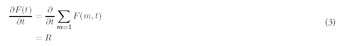
Let F(m, t) be the expected number of folds of a given size m at time t. The fold histogram determines both the expected total number of distinct folds F(t) and the expected total number of genes G(t):

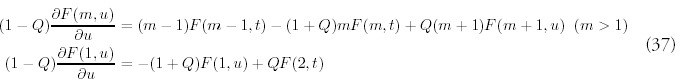
Under these growth assumptions, the Markovian dynamics governing F(m, t) are given by:

Although duplication occurs at the gene level, it is more convenient mathematically to work directly with the fold histogram F(m, t).

The intuition behind these equations is as follows. If the gene selected for duplication that originally is a member of a fold of size m — 1, then after duplication that fold will now be a fold of size m, and the population of F(m — 1,t) and F(m, t), will decrease and increase, respectively, by one. The probability for this particular gene selection is (m — 1)F(m —1,t)/G(t).

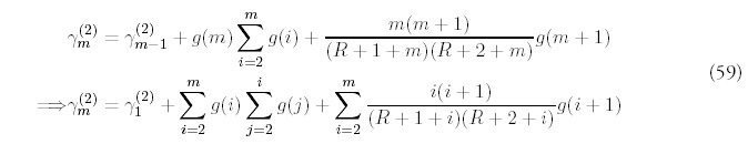
These equations ensure the appropriate expected growth rates for the total number of folds. A direct summation of (2) leads to:

The complete analytical solution for the coupled equations (2) can be found by standard methods. Full details are included in Appendix A.

The biological interpretation of the analytical solution is best appreciated by examining two important limiting cases. If there is no acquisition of new genes (R = 0), the solution simplifies considerably:

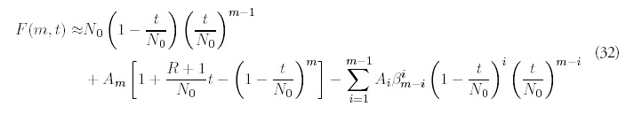
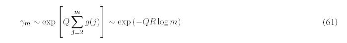
The other revealing limit concerns the behavior for large times (t → ∞)when new genes are acquired at a nonzero rate (R ≠ 0). The asymptotic limit is given by:

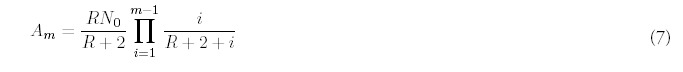
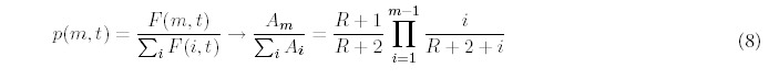
An examination of the leading large m behavior of A_m reveals that

It is also worth pointing that a power-law distribution that decays too slowly will lead to an infinite expected number of genes. A power-law distribution will that holds asymptotically for large m: N(m) ˜ 1/mα has to be described by an exponent α > 2 for the sum G(t) = m = ∑ mN (m) to converge. The asymptotic limit of the exact solution, a power-law with exponent R^m=1 + 2, satisfies this condition.

For nonzero R and times other than zero and infinity, the fold distribution will not be strictly exponential, nor will it conform to the limiting distribution (9). For small times, the analytic solution confirms what would be expected intuitively: the histogram behavior is dominated by duplication events involving the initial N₀ genes. To characterize the “crossover” behavior of the solution from the exponential to approximate power-law regime we have calculated the similarity of the exact probability distribution at different times to both the best fitting exponential distribution and to the limiting asymptotic distribution (9). The difference between any two probability distributions is measured by the sum of squared differences (the standard L² metric).

We have characterized the crossover time T_c for a range of values for both R and N₀ and find that the crossover time displays two distinct regimes. Within each regime it is approximately inversely proportional to R and directly proportional N₀: T_c˜ N0/R, with a different proportionality constant for each regime. Details of this analysis can be found in Appendix B. The numerical results indicate that crossover occurs roughly when the number of new fold introductions: RT_c, becomes comparable to the initial genome size N₀, as might be expected intuitively.

So far, we have assumed that the starting genome contains just one copy of each fold. In fact, it is reasonable to expect the initial genome to have several copies of particular fold types (for example those involved in protein synthesis) when the evolutionary process described by the model was initiated. By definition, genomes in our model have a comparatively small starting state, and so the difference between the most and least common folds would be minimal, i.e., some occurring three or four times at most. However, it is nonetheless of interest to investigate the effect that the appearance of the initial genome would have on the final distribution.

The solution we have derived for a particular initial genomic configuration—N₀ distinct folds consisting of one gene—can be extended to describe the evolution of an arbitrary initial fold distribution N_init(m) that is made up of N₀ genes: ∑_m mN_init(m) = N₀. The solution is similar to the special initial condition of N₀ distinct folds and is presented in detail in Appendix C.

One important conclusion may be drawn from the generalized model: all initial distributions ultimately lead to the same limiting distribution determined by the A_m. Just as before, the dependence on the initial fold distribution N_init(m) decays with time, leading to the same asymptotic distribution as was found for an initial distribution of N₀ folds of size 1 in (9), reflecting the dominance of fold introduction over gene duplication for large times. Of course, the details of how and when the crossover happens will depend on the particular form of N_init(m).

Extended Model: Including the Effects of Random Gene Deletion

Gene deletion is a major factor in evolution and is discussed briefly by Qian et al.¹¹ In this section we incorporate an additional parameter, Q, that represents gene deletion.

The most natural extension of (2) that accounts for random gene deletion at rate Q would be the following:

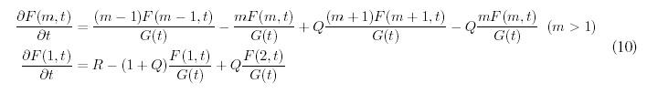
The terms proportional to Q encode the dynamics for gene deletion, which are very similar to gene duplication: on average, Q deletions occur for every duplication event and the gene to be deleted is chosen randomly from all the genes in the genome. In this way the population of a given bin m can either decrease due to gene deletion if the gene to be deleted is from bin m itself, or it can increase as a result of a deletion in the neighboring bin m + 1.

In this extended model, gene growth occurs at the uniform rate one would expect: G(t) = N₀ + (1 + R — Q)t. In contrast, the behavior of the expected number of folds is more complicated:

The extended model is much more complicated mathematically, primarily because the difference equations are now second order. In the minimal model, the behavior of larger folds depends only on the behavior of smaller folds, so the full solution can be constructed inductively starting from the solution for m = 1. With gene deletion operating as well, the dynamics of different fold sizes are coupled together. In many respects, these dynamics are like those describing diffusion phenomena; when Q = 0 the genome exhibits growth due to drift, or directed movement alone, while nonzero Q introduces diffusive, or non-directional movement as well.

Analytic Results

We were able to derive a full analytical solution only in the absence of any new fold introduction: R = 0. In this case, only stochastic gene deletion and duplication operate. We will restrict our discussion to when gene duplication occurs at a higher rate than gene deletion, which requires 0 < Q < 1, so the genome will still grow in size, at least in terms of number of genes: G(t) = N₀ +(1 — Q)t. Note that since R = 0, equation (11) shows that the number of folds will actually decrease with time. Losing folds while gaining genes is possible if the larger folds make up for the loss of genes from smaller folds.

An analytic solution exists for an initial distribution of N₀ different folds of size 1 and is worked out in detail in Appendix D. Once again, the distribution is exponential. Figure 3A shows histograms F(m,t) corresponding to three values of Q and a fixed time.

Figure 3

The effects of gene deletion: A) fold histogram F(m, t) for N₀ = 100 and t = 1000 plotted for Q = 0, 0.4, 0.8 and R = 0; B) normalized large-time limiting fold distribution and C) the total number of folds as a function of time when R = 1.0 and Q = 0, (more...)

Remarkably, the normalized distribution of fold size (the probability distribution) is independent of the gene deletion rate Q:

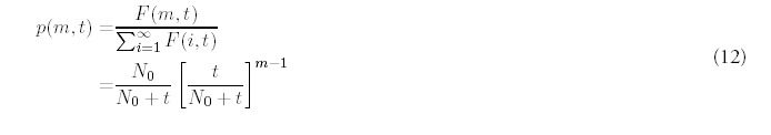
Hence gene deletion does not affect the shape of the distribution at all when R =0, only the overall normalization is changed. This can also be seen directly from Figure 3B.

Although an exact analytical solution does not seem possible for arbitrary R and Q, it is nonetheless possible to derive analytic expressions for the higher moments of the fold distribution. Appendix E discusses how this is done and particular, includes an expression for the second moment that will prove useful when fitting the model to genomic data.

Analytic Approximation Based on Perturbation Theory

The numerical results show that gene deletion, even for fairly large values of Q does not dramatically change the growth pattern of the genome, certainly qualitatively and to some extent, even quantitatively. Moreover, the analytic results when R = 0 showed that gene deletion is remarkably benign: in the absence of new gene acquisition, but with gene duplication operating, gene deletion does not change the probability distribution of fold occurrences, but does change expected total number of folds in the genome.

Here we consider an analytic approximation that attempts to capture the effects of gene deletion perturbatively by constructing an approximation around the Q = 0, R > 0 solution as an expansion in powers of Q. The perturbation expansion has to be handled carefully since a naive expansion, one that considers contributions only up to some finite power of Q, will not converge for all fold sizes m. The failure of conventional perturbation theory is explored in Appendix F.

To go beyond naive perturbation theory, we have adopted the following approach: (1) the dominant contribution at every order (or power) of Q is identified, (2) the dominant contribution is approximated, and (3) the resulting new infinite series in Q is summed exactly to arrive at an approximate solution that remains finite for all Q and m. The details are presented in Appendix F. Although not rigorous, this type of rescue or augmentation of perturbation theory is practiced routinely and often quite successfully on a variety physical models, such as models of phase transitions from statistical physics.²⁴

This approach leads to the following approximation for the limiting fold distribution:

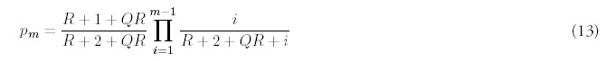
Note that the approximation includes as a special case the exact distribution derived previously for Q = 0 (8). In fact, the approximate distribution for Q nonzero is obtained from the exact solution for Q = 0 by the substituting R → R + QR. This correspondence also makes it clear that for large m, the Q ≠ 0 probability distribution will resemble a power law with exponent R + QR +2, just as Q = 0 distribution approached a power-law with exponent R + 2.

The true test of the effectiveness of the approximation rests with a comparison to the numerical results, which is done in Figure 3F. There seems to be good qualitative agreement, and fairly good quantitative agreement as well, even for Q = 0.4. As expected from the nature of the approximation, there is better agreement for large m in all cases. An approximation for the expected number of folds F(t) within the same framework is given in Appendix F.

The Effects of Selection Pressure

Selective pressure plays an important role in the evolution. It is well known that different genes have different duplication rate due to the selective pressure.²⁵ So far we have assumed that when genes are duplicated, or deleted, the target gene is chosen with equal probability from all the genes in the genome. A more realistic model would of course allow for favoritism in the selection process: presumably, genes that are useful or necessary are less likely to be deleted and perhaps more likely to be duplicated than genes that are less important. Note, however, that our model is not a differential survival model.

We explore the effects of selection pressure by extending the minimal model to allow for different duplication rates among genes. Suppose now that genes are not only identified with particular folds but also by their duplication types. For simplicity, assume that there are only two types: type “A” and type “B”, and that “B” genes are γ times more likely to be chosen for duplication than “A” genes. There will still be one duplication event, on average, per unit time, so the total expected number of genes will remain the same, but the allocation of the total between types “B” and “A” will depend on γ. We will assume that γ > 1, so it is the “B” types that are more likely to be duplicated.

To keep track of the fold population we now need two histograms: F_A(m, t) and F_B(m, t) to distinguish between the duplication types. The full fold histogram is the sum of both subhistograms: F(m, t) = F_A(m, t) + F_B(m, t). Similarly, let G_A(t) and G_B(t) represent the total number of genes for each type and define a new variable G_A(t):

The evolution equations that extend (2) are:

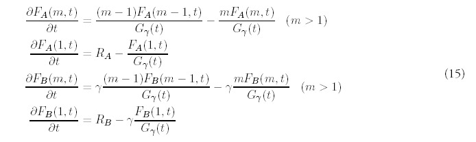
Note that we allow new folds to be acquired at different rates for each type: R_A can be different from R_B although we will restrict our numerical examples to the when they are equal.

The equations for the total number of genes of both types follow from the full dynamics (15) and are given in Appendix G. These confirm that the overall duplication rate is still one gene per unit time.

Once again, analytical solutions are possible for the two special parameter values addressed previously: (1) when there is no introduction of new folds, so R_A = R_B = 0; and (2) the limiting distribution when t → ∞. When there is no introduction of new folds, a simple extension of the methodology employed in Appendix A establishes that the each of the sub-histograms F_A(m, t) and F_B(m, t) follows an exponential distribution for all times. The full histogram is consequently a sum of exponential distributions:

The number of distinct folds of each type, present at t = 0 is given by N ^A0 and N ^B0. The variable u(t) is a rescaled time variable related to Gγ(t); the exact form of the dependence appears in Appendix G but is unimportant for the present discussion.

Of greater interest is the other special case: the ultimate evolutionary fate of the genome. The analytic behavior for large times is much easier to derive than an exact solution itself. For large t, G_γ(t) will grow linearly with time: G_γ ˜ t, according to a constant C_γ that depends on the rate of fold acquisition and the differential rate of duplication (see Appendix G for details).

In a similar fashion, we define coefficients C_m^A and C_m^B, akin to the coefficients A_m of the solution to the minimal model (7), that describe the ultimate linear growth of the histogram bins: F_A(m, t) ˜ C_m^At, and similarly for F_B(m, t). The normalized probability distribution corresponding to this limit is given by:

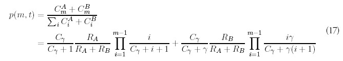
The important conclusion to be drawn from (17) is that powerlaw-like distributions describe the ultimate fate of the genome even when there are different rates of gene duplication. The probability distribution is the sum of two powerlaw-like distributions, each similar to the powerlaw-like distributions of the minimal model, but characterized by its own effective exponent. Figure 4 shows a comparison of the predicted distribution and numerical results when R_A = R_B = 0.5 for γ = 1, which is corresponds to the minimal model, and γ = 10, so type “B” genes are ten times more likely to be selected for duplication. The two distributions are remarkably close to each other, even when there is an order of magnitude difference between the relative duplication rates of type “B” genes. We have found that the parameter has much less of an effect than differences between the gene introduction rates R_A and R_B.

Figure 4

The effect of selective pressure on the model. Larger values of γ indicate larger differences in duplication rates between favored and unfavored protein folds. Large time limit for the fold probability distribution for γ = 1 and γ (more...)

We have also briefly considered the case of more than two duplication types. When there is no introduction of new folds into the genome equation (6) generalizes: the subhistogram for each duplication type is exponential. Furthermore, we have confirmed numerically that the terminal distribution is not dramatically affected by selection pressure, even when there are several families with significantly different rates of duplication. One particular example, involving four duplication types appears in Appendix G.

Fitting the Models to Genomic Data

Clearly, of greatest interest is to observe how our model compares with the genomic distributions. We start with the minimal model, for which we require estimates for the parameters t, N₀ and R for each organism.

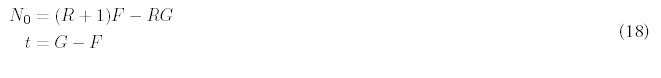
Fitting the minimal model requires estimating three parameters: t, N₀ and R. We have determined these parameters separately for each organism by insisting that the minimal model match the number of folds: F , the number of genes: G, and the second moment of the actual fold histogram: H₂, to those predicted by the minimal model. The fitting procedure is greatly simplified by the linear relation that exists between the variables (N₀, t) and (F, G):

The estimation of R is aided by recasting the expression for H₂ (Eq. 47 in Appendix D) so that t no longer appears explicitly. Instead, the second moment can be expressed so that it depends directly on F, G and the unknown R:

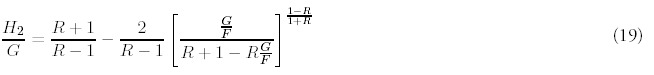
This equation is well behaved and can be easily solved numerically. What threatened to be a coupled, nonlinear three dimensional estimation problem is actually nothing more than a single nonlinear equation and two linear equations. We have verified that this fitting procedure accurately recovers parameters values from distributions generated both numerically and from the exact solution.

The results appear in Table 1. As a measure of the quality of the fit, we also report the mismatch of between the third moment predicted by the minimal model and observed in the data, as a percentage of the observed value; a positive value indicates that the model moment is larger. Plots of the actual fits appear in Figure 5.

Table 1

Fit of the minimal model using genomic data from 20 organisms.

Figure 5

Minimal model fits for A) C. elegans, B) A. fulgidus, C) M. tuberculosis, and D) M. genitalium using parameters from Table 1.

The parameter values are in fact very similar to those obtained in our previous work. The mismatch values range -13.1% to 9.9% and indicate that the distributions resulting from our model closely resembles the genomic distribution.

Our attempts to fit the models that included gene deletion were not that informative. This is partly because, as we have seen already, the gene deletion parameter Q does not have a dramatic effect on the shape of the distribution. We had difficulties even trying to fit distributions generated numerically from the extended model. Unlike the equations describing the minimal model, these coupled equations are also nonlinear. Furthermore, since there is no exact analytic expression for F(t), one of the variables itself has to be calculated numerically (We found that our analytic approximation for the number of folds given in Appendix F was not accurate enough to carry out the root-finding). We have found that naive multidimensional root-finding algorithms are either unable to distinguish between many approximate solutions, or find no solution at all at with increased sensitivity. The same difficulties were encountered in trying to discern evidence for selection pressure—there was too little dependence on the selection parameter γ to allow reliable estimation.

Conclusions

Here we propose two new models based on our previous model by fully incorporating two major processes in evolution: gene deletion and selective pressure. Both mathematically and biologically, including these effects are not slight. Mathematically, the derivations clearly show they are not trivial. Biologically, these effects provide a much more realistic model for genomic evolution than has been presented in any previous publications.^9,11,17 Furthermore, we provide analytical and numerical analyses of the original model and its extensions to explore the mathematical and biological significance of the models and to demonstrate the effects that the different evolutionary processes (gene duplication, acquisition, deletion and selective pressure) have on the final appearance of different genomes.

The field of the power-law distributions is controversial.^3-10,12,13 A number of fitting functions other than the power law were proposed to explain the observation. Our argument is that the question of which fitting function is the best should not be the central problem, because one can always find a function with more parameters fits the observation better than others.² Instead, we think biologically meaningful models are more helpful for understanding the origin of distribution and the analytical and numerical solutions shown in this work are vital for explaining the observation and further predicting the behaviour of the system.

The full analytical solution to this basic model revealed new facts that were unattainable from simulations only. As observed previously, gene duplication alone gives rise to an exponential distribution. However, the combined effect of duplication and acquisition changes the nature of genomic growth dramatically; beyond a sufficient length of evolutionary time, the fold distribution undergoes a transition from the exponential form, to a time-invariant limiting distribution that resembles a power law. The rate of fold acquisition (R) and the size of the initial genome (N₀) have distinct effects. Firstly, the cross-over time from the exponential to power-law phases is proportional to N₀ and approximately inversely proportional to R. This implies that the transition occurs when the number of new fold acquired becomes comparable to the initial size of the genome. Secondly, the decay rate of the power-law distribution i.e., the slope on a log-log plot is equal to R + 2 for large fold sizes. In fact, the final appearance of the distribution is independent of N₀, and is unaffected by the nature of the fold distribution in the starting genome. We find that the decay rate of the power-law distribution i.e., the slope on a log-log plot is equal to R + 2 for large fold sizes.

Note that we take R as a constant, and we regard this as the average rate of fold acquisition throughout the entire course of evolution. In reality, the value of R is likely to vary with time owing to a number of factors such as the decrease of available new protein folds. Further effects might be the increasing difficulty in horizontally transferring genes as the organism becomes more complex. These effects would generally lead to a decrease in rate of fold acquisition with time and this is perhaps reflected in the lower values of R for larger genomes.

We also studied extended models that fully incorporate the effects of random gene deletion and selective pressure. Gene deletion, represented by the parameter Q, does not significantly alter the qualitative behaviour found in the minimal model. The analytic solution showed that when there is no fold acquisition (R = 0), the distribution is again exponential and surprisingly, completely independent of Q. For cases where there is fold acquisition (R > 0), gene deletion had two main effects: firstly the final genome contained fewer fold types, and secondly all fold groups had smaller occurrences. Unsurprisingly, the extent of these effects was dependent on the size of Q. The final distribution nonetheless remains close to a power law, with a decay rate of R +2 + QR.

The effects of selective pressure were incorporated into the minimal model by introducing favouritism into the gene selection process. This was done by having two groups of genes, one with a higher probability of selection than the other. In this case, the two sets of genes effectively evolve with two distributions, each undergoing a transition from the exponential to power-law phases. Therefore, the final fold distribution is the sum of two power-law distributions, which in fact still closely resembles the distribution when no selective pressure is present. This is true even for large differences in duplication probabilities between the two sets of genes. More generally, we could imagine an array of finer differences in duplication probabilities representing the full range of selection pressures for genes of distinct biological functions. For this, we conjecture that selective pressure, at least when modelled as a duplication bias, will lead to folds that co-exist and compete for prominence in the genome, each undergoing separate, but linked distributional transformation.

We compared our minimal model compares with the genomic data by fitting parameter values. Figure 5 and the mismatch values in Table 1 show, the fits between the model and genomic data are good. As discussed in our earlier work, the parameters can be interpreted in a biologically meaningful way.¹¹ We did not use the new models for simulating biological data for two reasons: (1) they do not greatly affect the final appearance of the distribution; (2) if we would be trying to fit a model with three additional free parameters, this would detract from the main results of the paper.

In conclusion, although our model considers a few of the many important processes underlying genomic evolution, it is significant that a simplistic model based on gene duplication and fold acquisition leads to distributions close to those observed in genomic data. The current genomes provide only a snapshot in evolutionary time, but through our model, we gain a glimpse into the biological processes that are most important. Furthermore, by estimating parameter values, we obtain quantitative estimates such as the rate of gene acquisition, which would be otherwise unattainable. Interesting expansions to our model in future may include allowing parameter values to vary during the course of evolution, and modelling the evolution of different genomes simultaneously and simulating their divergence into different organisms.

Appendix A: Analytic Solution of the Minimal Model

It helps to introduce a new parameterization of time:

This new variable helps rid the differential equations (2) of explicit time dependence:

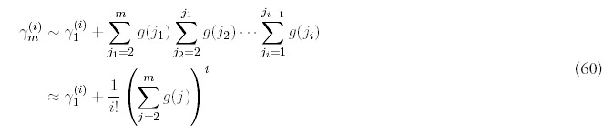
The solution for m = 1 can be found in the same way:

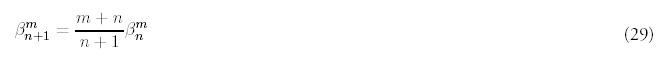
Note that the coefficients A_m and βnm do not depend on time, and furthermore has no dependence on R or N₀. The product of coefficients A_i βⁱ_m-1 can be simplified:

Figure 6

The normalized A_m coefficients (points) and a power-law fit (line), shown as a log-log plot as a function of size m, for R = 1.

Appendix B: Crossover Behavior

For nonzero R and times other than zero and infinity, the fold distribution will not be strictly exponential, nor will it conform to the limiting distribution (9). For small times, we would intuitively expect the histogram to be dominated by duplication events involving the initial N₀ genes. This is confirmed by the behavior of the analytic solution for small t:

There are many possible ways of characterizing this transformation of the fold distribution, each suggesting a different notion of a “crossover” time. We have looked at the convergence of the probability distribution as a whole. To quantify the extent to which the actual distribution p(m) resembles a second distribution, say p_A(m), we adopt the sum of the squared differences as our metric:

Figure 7

Crossover from exponential to large-time limiting distribution for R = 1.0 and N₀ = 100.

Figure 8 plots the crossover time as a function of R for two values of N₀. The range of R is chosen so that new fold acquisitions occur less frequently than (or as often as) gene duplication. The crossover time displays two distinct regimes. Within each regime it is approximately inversely proportional to R and directly proportional N₀. A different proportionality constant applies in each regime: T_c ˜ N₀/R. These numerical results confirm that crossover occurs roughly when the number of new fold introductions: RT_c becomes comparable to the initial genome size N₀. The details of the dependence are not that important, as they are no doubt strongly affected by the choice of metric.

Figure 8

Crossover time for N₀ = 100 and N₀ = 50, plotted as a function of A) R, and B) 1/R.

Appendix C: Arbitrary Initial Distribution

The solution for an arbitrary initial distribution: N_init(m), requires solving (2) subject to different boundary conditions at t = 0; the terms proportional to A_m are the same, the term proportional to N₀ is replaced by the superposition of new terms describing the propagation of each bin of initial histogram:

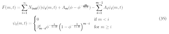
The fact that ψi(m,t) = 0 for m < i reflects the fact that there is no gene deletion; genes that start in bin i may either stay put or advance to bins corresponding to larger fold sizes, but will never populate bins of fold size less than i.

One important conclusion may be drawn from the full solution: all initial distributions ultimately lead to the same limiting distribution determined by the Am. Just as before, the dependence on the initial fold distribution Ninit(m) decays with time, leading to the same asymptotic distribution as was found for an initial distribution of N₀ folds of size 1 in Appendix A. Of course, the details of how the crossover happens will depend on the particular form of N_init(m).

Appendix D: Solution to the Extended Model When 0 < Q < 1 and R = 0

As one done in the solution for the minimal model, define Φ(t):

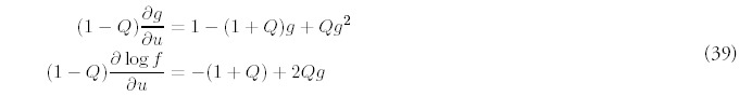
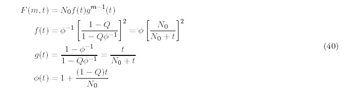
The large-time asymptotic limit for F(t) is (1 — Q)N₀ folds, which reflects the fact that some of the initial N₀ folds will ultimately be lost due to gene deletion. Equation (42) leads to a simple relation between the number of folds and the number of genes:

The solution (40) we have derived for 0 < Q < 1 is also the solution for Q = 1, which means that gene deletion and duplication occur at the same rate. Equations (42) and (43) for the total number of folds F(t) are still valid for Q = 1, but now the expected number of genes is constant: G(t) = N₀. Although we will not do so here, analytic solutions can be derived when deletion dominates duplication so the genome shrinks in size.

Appendix E: Analytical Results for Higher Moments

Higher moments of the distribution, defined as H_n(t) = ∑_m mⁿF(m, t), for n ≥ 2 in the extended model satisfy the following differential equation:

The solution for the second moment is given by:

Appendix F: Perturbation Theory Approximation for the Extended Model

As before, relate time and the number of genes through Φ(t):

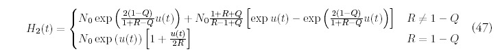
Recall that when Q = 0 and R > 0 the long-term behavior of F(m, t) is determined by the coefficients A_m, as shown in equation (30). Assume that the large-time solution in the presence of gene deletion is determined by new coefficients B_m:

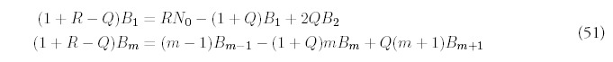
The remaining terms are determined order-by-order by substituting into (53) and collecting terms with the same power of Q:

The only way to obtain a consistent expansion is to sum all orders of the series. Unfortunately, the equations (55) are difficult to solve exactly, and even if they were possible to solve, it would be even more difficult to carry out the summation. However, it isn't difficult to figure out the dominant contribution at each order. It helps to first look at the equations for i = 2:

The same pattern emerges at all orders—the dominant contribution can be isolated as:

Motivated by this observation, and recalling that for large m, A_m ˜ 1/m^R+2 (from equation (8)), we suggest the following approximation for B_m, valid for all values of m, not just when m is large:

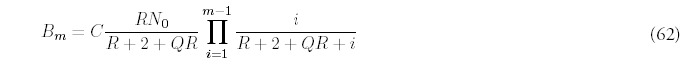
In order to determine F(t), the total number of folds at time t, equation (11) has to be solved using the approximate solution (62). First, the a choice has to be made for the constant C—since the equation is an approximation, there is freedom in the choice. One way is to enforce the consistency of equation (53) for m = 1:

Equation (11) can be integrated to give an approximation for F(t):

Figure 9 confirms these observations. The approximation for the expected number of folds seems to work quite well and could be useful in trying to infer both R and Q from genomic data. Certainly the impact of gene deletion is easier to identify through F(t) and G(t) than through the shape of the histogram F(m, t).

Figure 9

Analytic approximation for the total number of folds compared to numerical results of Figure 3.

Appendix G: The Effects of Selection Pressure

Recall that we have assumed that there are only two duplication types: type “A” and type “B”, and that “B” genes are γ times more likely to be chosen for duplication than “A” genes. There will still be one duplication event, on average, per unit time, so the total expected number of genes will remain the same, but the allocation of the total between types “B” and “A” will depend on γ. We will assume that γ > 1, so it is the “B” types that are more likely to be duplicated.

To keep track of the fold population we now need two histograms: F_A(m, t) and F_B (m, t) to distinguish between the duplication types. The full fold histogram is the sum of both subhistograms: F(m, t) = F_A(m, t) + F_B(m, t). Similarly, let G_A(t) and G_B(t) represent the total number of genes for each type and define a new variable Gγ(t):

As before, we derive equations for the total number of genes from the full dynamics (68):

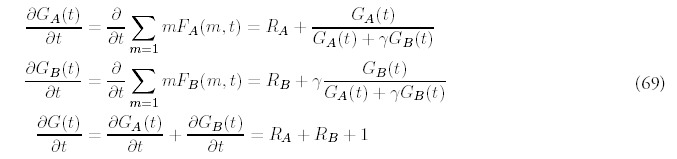
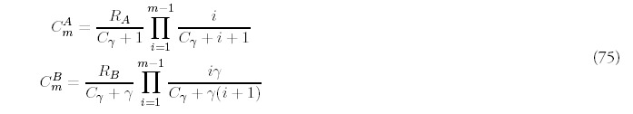
Figure 10

Large time limit for the fold probability distribution for the minimal model (one duplication type) and four duplication types: B = 4, C = 8, D = 16. The total rate of new fold acquisition is the same for both genomes.

Appendix H: A Useful Normalization Identity

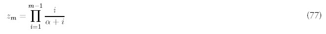
A series whose terms z_m, m =1, 2,... are defined by a recursion relation:

References

1.

Human Behaviour and the Principle of Least EffortIn: Zipf GK, ed.Cambridge: Addison-Wesley 1949.

2.

Luscombe NM, Qian J, Johnson T. et al. Power-law behaviour applies to a wide variety of genomic properties. Trends Genet, submitted. [PMC free article: PMC126234] [PubMed: 12186647]

3.

Mantegna RN, Buldyrev SV, Goldberger AL. et al. Linguistic features of noncoding DNA sequences. Phys Rev Lett. 1994;73(23):3169–72. [PubMed: 10057305]

4.

Konopka AK, Martindale C. Noncoding DNA, Zipf's law, and language. Science. 1995;268(5212):789. [PubMed: 7754361]

5.

Israeloff NE, Kagalenko M, Chan K. Can Zipf distinguish language from noise in noncoding DNA? Phys Rev Lett. 1996;1976 ;76(11) [PubMed: 10060571]

6.

Bonhoeffer S, Herz AV, Boerlijst MC. et al. No signs of hidden language in noncoding DNA. Phys Rev Lett. 1996;76:1977. [PubMed: 10060572]

7.

Voss RF. Comment on “Linguistic features of noncoding DNA sequences” Phys Rev Lett. 1996;76(11):1978. [PubMed: 10060573]

8.

Gerstein M. A structural census of genomes: Comparing bacterial, eukaryotic and archaeal genomes in terms of protein structure. J Mol Biol. 1997;274(4):562–76. [PubMed: 9417935]

9.

Huynen MA, van Nimwegen E. The frequency distribution of gene family sizes in complete genomes. Mol Biol Evol. 1998;15(5):583–9. [PubMed: 9580988]

10.

Koonin EV, Wolf YI, Aravind L. Protein fold recognition using sequence profiles and its application in structural genomics. Adv Protein Chem. 2000;54:245–75. [PubMed: 10829230]

11.

Qian J, Luscombe NM, Gerstein M. Protein family and fold occurrence in genomes: power-law behaviour and evolutionary model. J Mol Biol. 2001;313:673–681. [PubMed: 11697896]

12.

Jeong H, Tombor B, Albert R. et al. The large-scale organization of metabolic networks. Nature. 2000;407(6804):651–4. [PubMed: 11034217]

13.

Park J, Lappe M, Teichmann SA. Mapping protein family interactions: intramolecular and intermolecular protein family interaction repertoires in the PDB and yeast. J Mol Biol. 2001;307(3):929–38. [PubMed: 11273711]

14.

Rzhetsky A, Gomez SM. Birth of scale-free molecular networks and the number of distinct DNA and protein domains per genome. Bioinformatics. 2001;17(10):988–96. [PubMed: 11673244]

15.

Taverna DM, Goldstein RA. The distribution of structures in evolving protein populations. Biopolymers. 2000;53(1):1–8. [PubMed: 10644946]

16.

Shakhnovich EI. Protein design: a perspective from simple tractable models. Fold Des. 1998;3(3):R45–58. [PubMed: 9562552]

17.

Yanai I, Camacho CJ, DeLisi C. Predictions of gene family distributions in microbial genomes: evolution by gene duplication and modification. Phys Rev Lett. 2000;85(12):2641–4. [PubMed: 10978127]

18.

Lawrence JG, Ochman H. Molecular archaeology of the Escherichia coli genome. Proc Natl Acad Sci USA. 1998;95(16):9413–7. [PMC free article: PMC21352] [PubMed: 9689094]

19.

Doolittle WF. Phylogenetic classification and the universal tree. Science. 1999;284(5423):2124–9. [PubMed: 10381871]

20.

Ochman H, Lawrence JG, Groisman EA. Lateral gene transfer and the nature of bacterial innovation. Nature. 2000;405(6784):299–304. [PubMed: 10830951]

21.

Kidwell MG. Lateral transfer in natural populations of eukaryotes. Annu Rev Genet. 1993;27:235–56. [PubMed: 8122903]

22.

de la Cruz I, Davies I. Horizontal gene transfer and the origin of species: lessons from bacteria. Trends Microbiol. 2000;8(3):128–133. [PubMed: 10707066]

23.

LoConte L, Ailey B, Hubbard TJ. et al. SCOP: a structural classification of proteins database. Nucleic Acids Res. 2000;28(1):257–9. [PMC free article: PMC102479] [PubMed: 10592240]

24.

Statistical Field Theory, Vols. 1 and 2In: Itzykson C, Drouffe JM, eds. Cambridge: Cambridge University Press,1989.

25.

Protein EvolutionIn: Patthy L, ed.London: Blackwell Science 1999 .

26.

Differential Equations with Applications and Historical NotesIn: Simmons GF, ed.Englewood Cliffs: Prentice-Hall 1994.