Précis

Cancer in a particular tissue may progress by different pathways. Ideally, one would be able to measure progression and incidence separately for each pathway. In practice, observed incidence arises from combined progression over all pathways in a tissue. In this section, I analyze incidence and acceleration when aggregated over multiple underlying pathways of progression.

If one pathway progresses rapidly and another slowly, then incidence and acceleration will shift with age from dominance by the early pathway to dominance by the late pathway. For example, the early pathway may have few steps and low acceleration, whereas the late pathway may have many steps and high acceleration. Early in life, most cases arise from the early, low-acceleration pathway; late in life, most cases arise from the late, high-acceleration pathway.

In this example, the aggregate acceleration curve may be low early in life, rise to a peak in midlife when dominated by the later pathway, and then decline as the acceleration of the later pathway decays with advancing age. Aggregated pathways provide an alternative explanation for midlife peaks in acceleration. In the Conclusions at the end of this section, Figure 7.1 illustrates the main points and provides an intuitive sense of how multiple pathways affect incidence and acceleration. (Various multipathway models are scattered throughout the literature. See the references in Mao et al. (1998)).

Figure 7.1

Multiple pathways of progression in a tissue influence age-onset patterns of cancer. This figure shows epidemiological patterns for k = 3 pathways in a tissue in which there is a single line of progression, L = 1. On the y axis, the panels measure (a) (more...)

Details

For a particular tissue, I assume k distinct pathways to cancer indexed by j = 1,...,k. Each pathway has n_j transitions and i = 0,...,n_j states. The probability of being in state i of pathway j at age t is x_ji(t). A tissue is subdivided into L distinct lines of progression. A line might be a stem cell lineage, a compartment of the tissue, or some other architecturally defined component. Each line is an independent replicate of the system with all k distinct pathways.

Cancer arises if any of the Lk distinct pathways has reached its final state. All pathways begin in state 0 such that x_j0(0) = 1 and x_ji(0) = 0 for all i > 0. I interpret x_ji(t) as the probability that pathway j is in state i at time t.

The probability that a particular line progresses to malignancy is the probability that at least one pathway in that line has progressed to the final state,

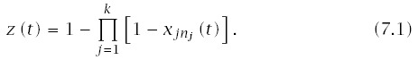
To keep the analysis simple, I focus on k pathways in one line. The solution for multiple lines scales up according to the theory outlined in Section 6.3. Typically, if the total probability of cancer, m, by age T is less than 0.2, then we have m/L ≈ z(T), and the cumulative probability of cancer at age t is p(t) ≈ z(t)L.

The transitions between stages are u_ji(t), the rate of flow in the jth pathway from stage i to stage i + 1. The transition rates may change with time. These distinct, time-varying rates provide the most general formulation. It is easy enough to keep the analysis at this level of generality, but then we have so many parameters and specific assumptions for each case that it becomes hard to see what novel contributions are made by having multiple pathways. To keep the emphasis on multiple pathways for this section, I assume that all transitions in each pathway are the same, u_j, that transition rates do not vary over time, and that distinct pathways indexed by j may have different transition rates.

Incidence at age t is

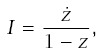
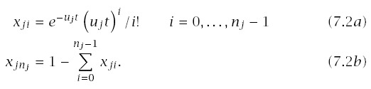
The rate of progression for a line is

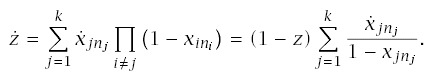
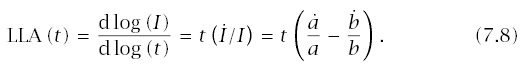
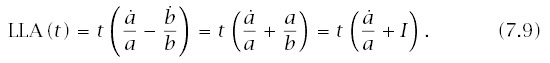
Using this formula for LLA to make calculations requires applying the pieces from earlier sections. In particular,

Conclusions

Figure 7.1 illustrates how multiple pathways affect epidemiological patterns. The pathway marked by the long-dash line in the figure shows a slowly accelerating cause of cancer that dominates early in life. The pathway marked by the dot-dash curve shows a rapidly accelerating cause of cancer that dominates late in life. The aggregate acceleration, shown by the sold curve in Figure 7.1b, is controlled early in life by the slowly accelerating pathway and late in life by the rapidly accelerating pathway. A pathway with intermediate acceleration, shown by the short-dash curve, contributes a significant number of cases through mid- and late life, but does not dominate at any age.

Précis

In the first case, one cannot distinguish between mutant and normal genotypes. If mutated genotypes are rare, then the aggregate pattern of incidence will be close to the pattern for the common genotype. A small increase in cases early in life does develop from the mutated genotypes, but those cases do not contribute enough to change significantly the aggregate pattern.

If the mutants are sufficiently frequent, they may change aggregate acceleration. Early in life, when mutants contribute a significant share of cases, aggregate acceleration may be dominated by the lower acceleration associated with mutants, which have fewer steps in progression than do normal genotypes. Late in life, aggregate acceleration will be dominated by the normal genotype, which has more steps and a higher acceleration. The net effect may be low acceleration early when dominated by the mutants, a rise to a midlife peak as dominance switches to the normal individuals, and a late-life decline in acceleration following the trend set by the normal genotype (Figure 7.2).

Figure 7.2

Genetic heterogeneity in the population influences aggregate epidemiological patterns. The rows, from top to bottom, are log-log incidence, log-log acceleration, and relative frequency of cancer caused by different genotypes. In each panel, the most common (more...)

In the second case, one can distinguish between mutant and normal genotypes. This is an important case, because it allows one to test directly the role of particular genes by comparison of mutant and normal patterns of incidence and acceleration. I show that the ratio, R, of normal to mutant incidence provides a good way to compare genotypes. The change in this ratio with age on log-log scales is the difference in acceleration between the normal and mutant genotype. Under simple models of progression dynamics, the observed difference in acceleration provides an estimate for the difference in the number of rate-limiting stages in progression.

Details

I assume a single pathway of progression in each line and a single line of progression per tissue, that is, k = L = 1. Extensions for multiple pathways and lines can be obtained by following the methods in prior sections. I assume the pathway of progression has n rate-limiting steps, with the transition rate between stages, u. Here, u is the same between all stages and does not vary with time.

A fraction of the population, p_j, has mutations that start them j steps along the pathway of progression; in other words, those individuals have n − j steps remaining before cancer. I refer to individuals that start j steps along as members of class j or as being born in the jth stage of progression.

AGGREGATE PATTERNS

If different genotypes cannot be distinguished, then all measurements on cancer incidence will combine the incidences for the different genotypes. The aggregate rate of transition into the final, cancerous state is

, where x_ji is the probability that an individual born in the jth stage has progressed a further i stages. The population-wide cumulative probability of having cancer by age t is z = ∑_{j = 0}^{n −1} p_jx_jn−j. Here, all values of z and x depend on time, but I have dropped the t to keep the notation simple. Eqs. (7.2) provide solutions for x_ji, substituting n − j for n_j, and noting the constant transition rates in this section, u_j = u for all j.

From these parts, we can write the total age-specific incidence in the population as

and the log-log acceleration as

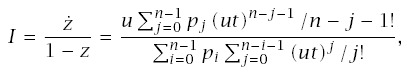
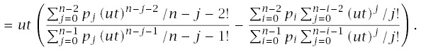
Figure 7.2 shows that genetic heterogeneity will typically have little effect on aggregate patterns of cancer. That figure assumes a common genotype with n = 10 steps and a rare mutant genotype with n−j steps, where j is the number of stages in progression by which the mutant genotype is advanced at birth. If the mutant advances only by j = 1, then the patterns differ little between the genotypes. If, however, n is small, as for retinoblastoma, then advancing one step, j = 1, can have a significant effect (not shown). Mutants are usually thought to advance progression by just one stage (Knudson 2001; Frank 2005), although relatively little direct evidence exists.

If mutants advance progression by j = 4 stages, then the mutants can have a significant impact on aggregate patterns, as shown in the middle column of Figure 7.2 in which the mutant occurs at a frequency of 0.01. However, the mutant must not be too rare—the right column of Figure 7.2 shows that genetic heterogeneity has little effect for j = 4, if the mutant occurs at a frequency of 0.001.

COMPARISON BETWEEN GENOTYPES: RATE-LIMITING STEPS

Mutant genotypes may often have little effect on aggregate pattern, as shown in the previous section. However, if one can track the incidence patterns separately for different genotypes, then much can be learned by comparison of incidence patterns between genotypes. Indeed, relative incidence patterns between genotypes may be the most powerful way to learn about cancer progression and the link between particular genes and cancer risk (Knudson 1993, 2001; Frank 2005).

In the next chapter, I will compare retinoblastoma incidence in humans between normal individuals and those who carry a mutation to the retinoblastoma (Rb) gene (Section 8.1). I will also compare colon cancer incidence between normal individuals and those who carry a mutation to the APC gene. In both cases, the ratio of age-specific incidences between normal and mutant individuals follows roughly along the curve predicted by multistage theory if the mutants begin life one stage further along in progression than do normal individuals (Frank 2005). Here, I develop the theory for predicting the ratio of incidences between normal and mutant genotypes.

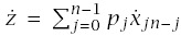
Assume a simple model of progression, with n stages and a constant rate of transition between stages, u. Mutant individuals begin life in stage j, and so have n − j stages to progress to cancer. The results of Section 6.2 provide the age-specific incidence for progression through n stages, I_n, so the ratio of incidences of normal and mutant individuals is

where S_j = ∑_{i = 0}^j (ut)ⁱ/i!.When j = 1, then R ≈ ut/(n − 1) is often a good approximation (Frank 2005).

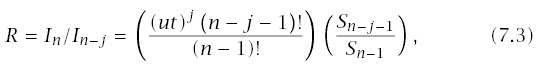
When comparing the incidences between two genotypes, it may often be useful to look at the slope of log(R) versus log(t), which is

where LLA_k, the log-log acceleration for a cancer with k stages, is given in Eq. (6.3). The slope of log(R) versus log(t) is equal to the difference in LLA, so I will sometimes refer to this slope as ΔLLA.

When progression causes acceleration to drop at later ages, then the slope of log(R) tends to decline with age. For example, in Figure 7.3, cancer develops through a single line of progression, L = 1. Often, a small number of progression lines tends to cause acceleration to drop at later ages. By contrast, in Figure 7.4, cancer develops through many lines of progression, L = 10⁸, which keeps acceleration nearly constant across all ages. Consequently, the ratio of incidences has a constant slope equal to the number of steps by which a mutation advances progression, that is,

Figure 7.3

Ratio of incidence rates between normal and mutant genotypes when there is a single line of progression, L = 1. The normal genotype has n steps in progression to cancer; the mutant has n − j steps. The top row shows the ratio on a log₁₀ scale, (more...)

Figure 7.4

Ratio of incidence rates between normal and mutant genotypes when there are multiple lines of progression. For these plots, L = 10⁸. To keep the cumulative probability at 0.1 for the normal genotype at age 80, u = 0.00052 for n = 5, and u = 0.00753 for (more...)

COMPARISON BETWEEN GENOTYPES: TRANSITION RATES

The previous section compared incidence rates between genotypes. In that case, one genotype required n steps to progress to cancer; the other mutant genotype inherited j mutations and began life with only n − j steps remaining. The inherited mutations abrogate rate-limiting steps.

In this section, I make a different comparison. Both genotypes require n steps to complete progression, but the mutant has a higher transition rate between stages. Let the transition rate for the normal genotype be u, and the transition rate for the mutant genotype be v = δu, with δ > 1. As in Eq. (7.4), I calculate the log-log slope of the ratio of incidences, in this case taking the ratio of mutant to normal genotypes, R. The solution follows from Eq. (6.3):

where S^α_j = ∑^j_{i= 0} (αt)ⁱ/i!

Figure 7.5 illustrates this theory. The left column shows the standard log-log incidence curves. The bottom curve plots the wild-type incidence; the curves above show incidence for mutants with higher transition rates. The right column plots the difference in the slopes of the incidence curves, ΔLLA, between the wild-type and the various mutant genotypes.

Figure 7.5

Comparison between genotypes with different transition rates. (ad) The left incidence panels show the standard log-log plot, with incidence on a log₁₀ scale. The bottom, short-dash curve in each incidence panel illustrates the wild-type genotype. The (more...)

The bottom right panel, Figure 7.5h, uses L = 10⁸ independent lines of progression within the tissue under study. With large L, almost all lineages remain in the initial stage throughout life and have n stages remaining; thus, the log-log incidence slopes remain near n−1 for both wild-type and mutant genotypes.

The top right panel, Figure 7.5e, uses L = 10⁰ independent lines of progression within the tissue. With small L, the few lineages at risk tend to progress with age through at least the early stages, causing a reduction in the number of remaining stages and a drop in the log-log incidence slope. The mutants, with faster transition rates, advance more quickly through the early stages and so, at a particular age, have fewer stages remaining to cancer. With fewer stages remaining, those mutants have lower log-log incidence slopes, and therefore the difference in slopes, ΔLLA, between wild-type and mutant genotypes increases. Figure 7.5 uses n = 7 stages; Figure 7.6 provides similar plots but with n = 10 stages.

Figure 7.6

Comparison between genotypes with different transition rates. Assumptions are the same as in Figure 7.5, except that n = 10 and δ = 3^i/4 for i = 1,...,4.

In summary, a mutant genotype that increases transition rates will cause a rise in ΔLLA when compared with the wild type. This increase in ΔLLA occurs even though the number of rate-limiting stages is the same for mutant and wild-type genotypes. The amount of the rise with age in ΔLLA depends most strongly on the increase in transition rates caused by the mutant and on the number of independent lines of progression in the tissue.

Conclusions

The ratio of normal to mutant incidence provides one of the best tests for the role of genetics in progression dynamics. Figures 7.3 and 7.4 show predictions for this ratio under simple assumptions about progression. Similar predictions could be derived by analyzing the ratio of incidences in other models of progression, such as those developed in earlier sections. In Chapter 8, I analyze data on the observed ratio of incidences between normal and mutant genotypes. Those ratio tests provide the most compelling evidence available that particular inherited mutations reduce the number of rate-limiting stages in progression.

Précis

I use the basic model of multistage progression, in which carcinogenesis proceeds through n stages, and each individual has a constant rate of transition between stages, u. To study heterogeneity, I assume that u varies between individuals. Both genetic and environmental factors contribute to variation.

There are L independent lines of progression within each individual, as described in Section 6.3. I use a large value, L = 10⁷, which causes log-log acceleration (LLA) to be close to n−1, without a significant decline in acceleration late in life (Figure 6.1).

To analyze variation in transition rates between individuals, I assume that the logarithm of u has a normal distribution with mean m and standard deviation s. This sort of log-normal distribution often occurs for quantitative traits that depend on multiplicative effects of different genes and environmental factors (Limpert et al. 2001).

Figure 7.7 shows examples of log-normal distributions. Note that a small fraction of individuals has large values relative to the typical member of the population. In terms of cancer, such individuals would be fast progressors and would contribute a large fraction of the total cases.

Figure 7.7

The log-normal probability distribution used to describe variation in transition rates, u. (a) In a log-normal distribution of u, the variable ln(u) has a normal distribution with mean m and standard deviation s. The three solid curves show the distributions (more...)

The question here is: How does heterogeneity influence epidemiological pattern? To study this, I increase variability by raising the parameter s in the log-normal distribution, which increases the variability in transition rates, u. To measure epidemiological pattern, I analyze how changes in s affect log-log acceleration.

Figure 7.8 shows that increasing variability causes a large decline in acceleration when epidemiological pattern is measured over the whole population. In this example, s measures variability: in the top curve, s = 0 and the population contains no variability; in the second curve from the top, s = 0.2, showing the effect of a small amount of variability; the curves below increase variability with values of s = 0.4,0.6,0.8,1.0, respectively.

Figure 7.8

Acceleration for different levels of phenotypic heterogeneity in transition rates. Each curve shows the acceleration in the population when aggregated over all individuals, calculated by Eq. (7.9). I used a log-normal distribution for f(u) to describe (more...)

In Figure 7.8, focus on the curve labeled s = 0.6. That curve shows the acceleration of cancer in the total population. Figure 7.9 illustrates the contribution to that aggregate curve by different subgroups of the population with different values of the transition rate, u.

Figure 7.9

Explanation of the drop in aggregate acceleration caused by population heterogeneity. Each panel shows patterns for different segments of the population stratified by transition value, u. The legend in (a) shows that each of the first four strata comprise (more...)

Figure 7.9a plots the contribution of each subgroup in the population: the sum of the individual curves determines the aggregate curve in Figure 7.8. At different ages, each subgroup contributes differently to the aggregate pattern. The solid curve shows the top 2.5% of the population with the highest values of u, defined in the legend as the group between the 97.5th percentile and the 100th percentile. The legend gives the percentile levels for the other curves.

In Figure 7.9a, the solid curve shows that those who progress the fastest contribute most strongly to acceleration early in life. In Figure 7.9b, the solid curve shows the fraction of individuals in that group who have progressed to cancer; already by age 30, ten percent of that group has developed cancer, and by age 60, nearly everyone in that group has progressed.

Returning to Figure 7.8a, we can see that, as age increases, successive groups rise and fall in their contributions to total acceleration in the population. The contribution of each group peaks as the fraction of individuals affected in that group increases above ten percent (Figure 7.9b), and then the contribution declines as nearly all individuals in the group progress to cancer.

Figure 7.9c shows the acceleration pattern if each subgroup were itself the total population. Each group is itself heterogeneous, but with variation over a smaller scale than in the aggregate population. The acceleration pattern is relatively high and constant within all groups except the two highest groups, comprising 5% of the population, who progress very fast.

Figure 7.9b shows that under heterogeneity, cancer forms a rather sharp boundary between those strongly prone to disease, who progress with near certainty, and those less prone, who progress with low probability. This kind of sharp cutoff between those affected and those who escape is sometimes called truncation selection.

The truncating nature of selection in this example can also be seen in Figure 7.7, in which the dotted line measures the probability that an individual will have progressed to cancer by age 80 (right scale). Those few individuals with higher u values progress with near certainty; the rest, with lower u values, rarely progress to cancer. The transition is fairly sharp between those values of u that lead to cancer and those values that do not.

Details

I assume a single pathway of progression in each line, k = 1, and allow multiple lines of progression per tissue, L ≥ 1. Extensions for multiple pathways can be obtained by following the methods in earlier sections. I assume the pathway of progression has n rate-limiting steps with transition rate between stages, u. Here, u is the same between all stages and does not vary with time. Each individual in the population has a constant value u in all lines of progression. The value of u varies between individuals. In this case, u is a continuous random variable with probability distribution f(u).

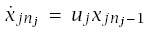
I obtain expressions for incidence and log-log acceleration that account for the continuous variation in u between individuals. To start, let the probability that a particular line of progression is in stage i at time t be x_i(t,u), for i = 0,...,n. For a fixed value of u, we have from Section 6.2 that x_i(t,u) = e^−ut(ut)ⁱ/i! for i = 0,...,n − 1 and x_n(t,u) = 1 − ∑ⁿ⁻¹_i=0 x_i(t,u).

The probability that an individual has cancer by age t is the probability that at least one of the L lines has progressed to stage n, which from Eq. (6.5) is

Incidence is the rate at which individuals progress to the cancerous state divided by the fraction of the population that has not yet progressed to cancer. The rate at which an individual progresses is

The fraction of the population that has not yet progressed to cancer is

With these expressions, incidence is I(t) = a/b, and log-log acceleration is

To make calculations, we need to express a and

Conclusions

Increasing heterogeneity causes a strong decline in the acceleration of cancer. Heterogeneity could, for example, cause a cancer with n = 10 stages to have acceleration values below 5 that decline with age. Thus, low values of acceleration (slopes of incidences curves) do not imply a limited number of stages in progression. Heterogeneity must be nearly universal in natural populations, so heterogeneity should be analyzed when trying to understand differences in epidemiological patterns between populations.

Heterogeneity in progression rates causes cancer to be a form of truncation selection, in which those above a threshold almost certainly develop cancer and those below a threshold rarely develop cancer. Under truncation selection, the amount of variation in progression rates will play a more important role than the average rate of progression in determining what fraction of the population develops cancer and at what ages they do so. To understand the distribution of cancer, it may be more important to measure heterogeneity than to measure the average value of processes that determine rates of progression.

Précis

Demographers and engineers use Weibull and Gompertz models to describe age-specific mortality and failure rates. A simple form of the Weibull model assumes that failure rates versus age fit a straight line on log-log scales. This matches the simplest multistage model of progression dynamics under the assumption that log-log acceleration remains constant over all ages.

The advantage of the Weibull model is that it makes no assumptions about underlying process, and allows one to reduce data description to the two parameters of slope and intercept that describe a line. Comparison between data sets can be made by comparing the slope and intercept estimates.

The disadvantage of the Weibull model is that, because it is a descriptive model that makes no assumptions about underlying process, one cannot easily test hypotheses about how particular factors affect the processes of progression. I prefer an explicit underlying model of progression dynamics. In some cases, such as the simplest multistage model, the solution based on explicit assumptions about progression leads to an approximate Weibull model.

The common form of the Gompertz model arises by assuming a constant value for the slope of incidence versus age on log-linear scales: that is, logarithmic in incidence and linear in age. The advantages and disadvantages for the Weibull model also apply to the Gompertz model.

Details

The Weibull model describes age-specific failure rates. Engineers use the Weibull model to analyze time to failure for complex control systems, particularly where system reliability depends on multiple subcomponents. Multicomponent failure models have a close affinity to multistage models of disease progression. Demographers also use the Weibull model to describe the rise in age-specific mortality rates with increasing age.

Both engineers and demographers have observed that the Weibull model provides a good description of age-specific failure rates in many situations, so they use the model to fit data and reduce pattern description to a few simple parameters. Various forms of the Weibull model exist. A simple and widely applied form can be written as

The simple model of multistage progression with equal transition rates, given in Eq. (6.2), can be rewritten as

If I(t) ≈ αt^β is a good approximation of the observed pattern of age-specific incidence, then multistage progression dynamics approximately follows the Weibull model. On a log-log scale, the relation is

Whenever log-log acceleration remains constant with age, the multistage and Weibull models will be similar. The previous sections discussed the assumptions under which log-log acceleration remains constant with age.

The Weibull model simply describes pattern, and so cannot be used to develop testable predictions about the processes that control age-specific rates. With multistage models of progression, we can predict how incidence will change in individuals with inherited mutations compared with normal individuals, or how incidences of different diseases compare based on the number of stages of progression, the number of independent lines of progression, the variation in transition rates between stages, and the temporal changes in transition rates over a lifetime.

The Gompertz model provides a widely used alternative description of mortality rates. Let G(t) be the age-specific mortality rate of a Gompertz model, and let a dot denote the derivative with respect to t. The Gompertz model assumes that the mortality rate increases at a constant rate γ with age:

The Gompertz model arises when one assumes a constant life table aging rate. As with the Weibull model, the Gompertz model describes the pattern that follows from a simple assumption about age-related changes in failure rates. Neither model provides insight into the processes that influence age-related changes in disease. However, these models can be useful when analyzing certain kinds of data. For example, the observed age-specific incidence curves may be based on relatively few observations. With relatively few data, it may be best to estimate only the slope and intercept for the incidence curves and not try to estimate nonlinearities.

When fitting a straight line on a log-log scale, one is estimating Weibull parameters. Similarly, fitting a straight line of incidence versus time on a log-linear scale estimates parameters from a Gompertz model. The Weibull distribution may be the better choice because it provides a linear approximation to an underlying model of multistage progression dynamics.

Conclusions

Weibull and Gompertz models provide useful tools to reduce data to a small number of estimated parameters. However, I prefer to begin with an explicit model of progression dynamics and derive the predicted shape of the incidence curve. Explicit dynamical models allow one to test comparative hypotheses about the processes that influence progression.

Précis

Peto et al. (1991) provided the most comprehensive experiment and analysis of carcinogen dose-response curves. In their analysis, they compared the observed age-specific incidence of cancer (the response) over varying dosage levels. They described the incidence curves by fitting the data to the Weibull distribution. They also related the Weibull incidence pattern to the classic Druckrey formula for carcinogen dose-response relations. The Druckrey formula summarizes the many carcinogen experiments that give linear dose-response curves when plotting the median time to tumor onset versus dosage of the carcinogen on log-log scales (Druckrey 1967).

I discussed the Druckrey equation, the data from Peto et al.'s study, and some experimental results from other carcinogen experiments in Section 2.5. Here, I summarize the theory that ties the Weibull approximation for incidence curves to the Druckrey equation between carcinogens and tumor incidence.

Details

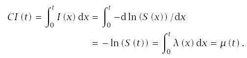
Define the instantaneous failure rate asλ(t). Cumulative failure intensity is μ(t) = ∫^t₀ λ(x)dx. Then, from the nonstationary Poisson process, the probability of survival (nonfailure) to age t is

Note that median time to failure, m, is

Age-specific incidence, I(t), is the instantaneous decrease in survival divided by the fraction of the original population still surviving, thus

Cumulative incidence sums up the age-specific incidences; cumulative incidence measures the total failure intensity over the total time period, thus

This background provides the details needed to decipher the rather cryptic analysis in Peto et al. (1991) on the Weibull distribution and the Druckrey equation.

To start, assume that cumulative failure follows the Weibull distribution

Thus, the median, m, and the exponent, n, completely determine the course of survival, time to failure, and incidence.

For carcinogen experiments, Druckrey and others have noted an excellent linear fit on log-log scales between the median time to tumor, m, and dosage, d, such that

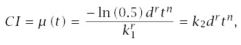
Note that if d = 0, this formula for incidence suggests no cancer in the absence of carcinogen exposure. If there is a moderate to high dosage, then almost all cancers will be excess cases induced by carcinogens. However, one may wish to correct for background cases, either by interpreting CI as excess incidence or by substituting (d + δ)^r for d, where δ > 0 explains the background cases.

Conclusions

This section provided the technical details to analyze experimental studies of carcinogens. Those studies measure the relation between tumor incidence and age at different dosage levels. The analysis then estimates the effect of dosage on the time to tumor development. Most studies fit well to a model in which the cumulative incidence up to age t rises with d^rtⁿ, where d is dose, t is age, the exponent r is the log-log slope for incidence versus dosage, and n is the log-log slope for cumulative incidence versus age.